from timeit import default_timer as timer
import math
import random
random.seed(1337) #To repeat results
We are going to go through the fundamentals of Neural Networks by solving the MNIST Handwritten Digits dataset without using any external libraries and creating a simple multilayer perception. That’s right, we’re just going to use the base installation of Python, so it’s going to be iterative and veeerrry slow. Due to this we’ll simplify and shorten some things, however we’ll still achieve ~90% accuracy. This is the first instance of a 4-part series of solving this dataset which will build upon the fundamentals of Neural Networks as we add more cutting edge techniques and build upon this network. In part 1 here we’ll learn what a Neural Network is and how it works at its most fundamental level through backpropagation and we’re going to gain a great appreciation for vectorization after we see how long it takes to train this simple network without it. Additionally, we won’t be creating any Python Classes or Functions or do any fancy Pythonic one-liners which should keep this very beginner friendly and easy to read through!
So first off, what is a Neural Network? Well, I could attempt to explain them through text and some images, but honestly as someone who’s been a total beginner and tried to first learn about them by reading articles and Wikipedia pages that was just a waste of time in hindsight… Instead, let me point you to what I wish someone had for me back then: 3Blue1Brown’s Neural Network series on YouTube. Now, I know this is a bit of a cop-out, but trust me, no amount of text and pictures can do a better job then this video series. This visual-focused series was incredible for obtaining that intuative fundamental understanding which creates a solid base for further learning, so if you’re a newbie then I definitely recommend checking it out. That said, I’ll add my own descriptive intuition on top:
>Neural Networks are a fairly naive mimic of how our incredibly complex brains’ work. We see, hear, feel, etc some input which is processed by our brain (the hidden layers) and our reaction to it is the output. Since everything in our universe can be described by functions and math we are able to replicate this with Neural Networks which are also known as “universal function approximators”. When broken down into their smallest parts (nodes), they are actually fairly simple mathematical operations. It’s how all these simple operations are connected to each other which makes them complex as a whole. This is analogous to how our digital lives are all based upon simple “on’s” and “off’s”, i.e. Zeros and Ones, which are all interconnected to create far more complex outputs such as this text right here. In Neural Networks however, instead of zeros and ones there are simple functions like the familiar y = mx + b all intertwined where together in large quantities can do amazing things.
Now that you’ve got a little intuition of how these networks work, let’s build one from scratch!
We shall start by importing the only libraries we need which are all part of the base Python 3.7 installation:
We will be training on the MNIST dataset which consists of 70,000 28px by 28px grayscale images of handwritten digits from 0-9. The goal is to train a network on this data and later be able to input a new (not seen before by the network) image of a digit and properly output the correct number of said image. In an effort to keep things as simple as possible we’ll be using the CSV version of this database found here. The data is split up into 60,000 images for training and 10,000 images for testing. Let’s open it:
train_data = open('mnist_train.csv', 'r').read().splitlines()
test_data = open('mnist_test.csv', 'r').read().splitlines()
Let’s briefly look at a portion of the first two lines of train_data. We can see the first line is header information and tells us that the first value of each subsequent line is the label for the digit image. We also see the expected pixel values from 0 (black) to 255 (white):
print(train_data[0][0:100])
print(train_data[1][0:400])
label,1x1,1x2,1x3,1x4,1x5,1x6,1x7,1x8,1x9,1x10,1x11,1x12,1x13,1x14,1x15,1x16,1x17,1x18,1x19,1x20,1x2
5,0,0,0,0,0,0,0,0,0,0,0,0,0,0,0,0,0,0,0,0,0,0,0,0,0,0,0,0,0,0,0,0,0,0,0,0,0,0,0,0,0,0,0,0,0,0,0,0,0,0,0,0,0,0,0,0,0,0,0,0,0,0,0,0,0,0,0,0,0,0,0,0,0,0,0,0,0,0,0,0,0,0,0,0,0,0,0,0,0,0,0,0,0,0,0,0,0,0,0,0,0,0,0,0,0,0,0,0,0,0,0,0,0,0,0,0,0,0,0,0,0,0,0,0,0,0,0,0,0,0,0,0,0,0,0,0,0,0,0,0,0,0,0,0,0,0,0,0,0,0,0,0,3,18,18,18,126,136,175,26,166,255,247,127,0,0,0,0,0,0,0,0,0,0,0,0,30,36,94,154,170,253,253,253Now we need to convert this data into Python lists to work with. X_train, Y_train, X_test, Y_test are standard variable names for our data. We’ll start by skipping that first header line and then splitting lines by each comma and using the map() function to convert them all from Strings to Integers. Then we’ll append each label and array of pixel values to train and test lists:
X_train_full, Y_train_label_full = [], []
for line in train_data[1:]:
    #Split CVS by comma and map each String Value to Int:
    num_array = list(map(int, line.split(',')))
    #num_array then has the first index as Label, and remaining as Pixel data.
    Y_train_label_full.append(num_array[0])
    X_train_full.append(num_array[1:])
#Do the exact same for the testing data:
X_test_full, Y_test_label_full = [], []
for line in test_data[1:]:
    num_array = list(map(int, line.split(',')))
    Y_test_label_full.append(num_array[0])
    X_test_full.append(num_array[1:])
Since we’re going to be using an inefficient iterative approach in this part of the series, we’ll randomly drop 90% of the data and keep only 10%. Even with only 10% of the data, there will still be a heckin’ lot of iterations so training will take a long time. We’ve imported a timer to see just how long it’ll take to train up to 90% accuracy and then in part 2 we’ll use vectorization with 100% of the data to really illustrate just how important vectorized solutions are and how they’re essentially why Machine Learning has been able to advance so much.
#Keep only 10% of the data, randomly
data_drop = 10
#First, the Training Data
rnd_idxs = list(range(len(X_train_full)))
random.shuffle(rnd_idxs)
X_train, Y_train_label = [], []
for i in range(len(X_train_full)//data_drop):
    X_train.append(X_train_full[rnd_idxs[i]])
    Y_train_label.append(Y_train_label_full[rnd_idxs[i]])
#And then the test data:
rnd_idxs = list(range(len(X_test_full)))
random.shuffle(rnd_idxs)
X_test, Y_test_label = [], []
for i in range(len(X_test_full)//data_drop):
    X_test.append(X_test_full[rnd_idxs[i]])
    Y_test_label.append(Y_test_label_full[rnd_idxs[i]])
#Remove these from memory as we will no longer use them:
del X_train_full
del Y_train_label_full
del X_test_full
del Y_test_label_full
Let’s see what we’ve got! Each 28px by 28px image is now a 28x28 = 784 length array and we have 6000 training images with 1000 test images:
img_pxs = len(X_train[0])
total_train = len(Y_train_label)
total_test = len(Y_test_label)
print(f'Total pixels per image: {img_pxs}')
print(f'Total images to train on: {total_train}')
print(f'Total images to test with: {total_test}')
Total pixels per image: 784
Total images to train on: 6000
Total images to test with: 1000It is always a good idea to visualize your data, especially to confirm that you’re setup properly. To do this we’re going to cheat a little and use the external library matplotlib just for this cell so we can convert our pixel arrays into images:
%matplotlib inline
import matplotlib.pyplot as plt
fig, axes = plt.subplots(ncols=10, figsize=(10, 10))
for i in range(10):
    data_test = []
    last = 0
    for j in range(int(img_pxs**0.5), img_pxs + 1, int(img_pxs**0.5)):
        data_test.append(X_train[i][last:j])
        last = j
    axes[i].imshow(data_test, cmap="gray")
    axes[i].axis('off')
    axes[i].set_title(Y_train_label[i])
print('First 10 labels and images:')
plt.show()
First 10 labels and images: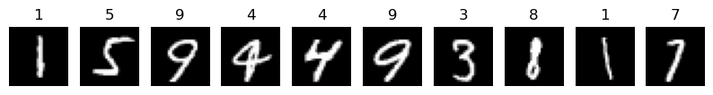
It is also wise to normalize your data. There are many reasons for this such as to increase training speed or preventing gradient descent from getting stuck in local optima. In general though, it’s standard practice to normalize all your data especially if you have different features which do not all have the same scale. For this image case, we simply divide every pixel by the largest, 255:
#normalize the X data between 0 and 1:
for img_idx, img_arr in enumerate(X_train):
    for px_idx, px_val in enumerate(img_arr):
        X_train[img_idx][px_idx] = px_val/255
for img_idx, img_arr in enumerate(X_test):
    for px_idx, px_val in enumerate(img_arr):
        X_test[img_idx][px_idx] = px_val/255
The output of a classification Neural Network is a list of probabilities. In our case when classifying 10 digits, we will need an output list of 10 probabilities which each correspond to each digit where the highest is the network’s predicted label. Therefore, to be able to compare this to the true label of each image we need these labels converted into lists of size 10 where the index of the true label is a 1 for 100% probability and the rest are 0. This is also known as one-hot encoding:
label_encode_dict = {0: [1, 0, 0, 0, 0, 0, 0, 0, 0, 0],
                     1: [0, 1, 0, 0, 0, 0, 0, 0, 0, 0],
                     2: [0, 0, 1, 0, 0, 0, 0, 0, 0, 0],
                     3: [0, 0, 0, 1, 0, 0, 0, 0, 0, 0],
                     4: [0, 0, 0, 0, 1, 0, 0, 0, 0, 0],
                     5: [0, 0, 0, 0, 0, 1, 0, 0, 0, 0],
                     6: [0, 0, 0, 0, 0, 0, 1, 0, 0, 0],
                     7: [0, 0, 0, 0, 0, 0, 0, 1, 0, 0],
                     8: [0, 0, 0, 0, 0, 0, 0, 0, 1, 0],
                     9: [0, 0, 0, 0, 0, 0, 0, 0, 0, 1],}
Y_train, Y_test = [], []
for i in range(len(Y_train_label)):
    Y_train.append(label_encode_dict[Y_train_label[i]])
for i in range(len(Y_test_label)):
    Y_test.append(label_encode_dict[Y_test_label[i]])
Now that we have our train and test data all ready, we can initalize our simple network. For this inefficient approach with only 10% of the data we’re going to create a relatively small network of just one hidden layer and an output layer. Our hidden layer will have 32 nodes and then of course the output layer will need 10 nodes, for classifying 10 digits. The initial weights of a network are actually quite important. If they’re all zero then no training will occur, if they’re too small then training takes forever and the gradient can vanish, and finally if they’re too large then then the training is fairly eradict and the gradient can actually explode, i.e. oscillate around the minimum we hope to find. Additionally, if weights are all uniform then training greatly suffers because during backpropagation changes to all the weight will have identical infulence on the cost. Deeplearning.ai has a great tool to visualize what happens during training when networks are initalized both poorly and correctly. To follow best practice, even though we’re not creating a deep neural network here, we’re going to setup the network using the Xavier initalization where each layer will have a random, but uniform, range of values between \(-\frac{1}{\sqrt{i}}\) to \(\frac{1}{\sqrt{i}}\) where \(i\) is the number of inputs to the layer.
Nodes are also often referred to as neurons, which honestly sounds so much cooler so let’s use that term! So for our first and only hidden layer consisting of 32 neurons, we have each image which has been converted into a 784 data array (and is each row in X_train) that will be the input to this layer and we want each neuron, whether it “fires” or not, to have a single output. Therefore, we have 784 inputs with 32 outputs meaning we want to initalize the first weight matrix, W1, to be of size 784 by 32. Additionally, will want a bias for each neuron which we can initalize to be 0; so since we’ve got 32 neurons we’ll create a 1 by 32 bias matrix, b1:
#Hidden layer - 784 input by 32 output
layer1_in = img_pxs
layer1_out = 32
b1 = [0]*layer1_out #initalize bias to 0
W1 = []
for i in range(layer1_in):
    W1_row = []
    for j in range(layer1_out):
        #Using Xavier initalization...
        Xav_upper = 1.0/math.sqrt(layer1_in)
        Xav_lower = -1.0/math.sqrt(layer1_in)
        r_num = random.uniform(Xav_lower, Xav_upper)
        W1_row.append(r_num)
    W1.append(W1_row)
For our second layer, which is our output layer, we have 10 neurons each relating to the probability of each of the 0-9 digits, respectively. The highest neuron will be the digit the network thinks the initial image input is. Since we had 32 neurons in the previous layer, which means there’s 32 outputs from that layer, we will have 32 inputs into this next layer. So, similar to the previous layer we will initalize the second weight matrix, W2, to be of size 32 by 10 and then create a second bias matrix full of 0’s of size 1 by 10:
#Output layer - 32 input by 10 output
layer2_in = layer1_out
layer2_out = 10 # 10 digit prediction output
W2 = []
b2 = [0]*layer2_out #initalize bias to 0
for i in range(layer2_in):
    W2_row = []
    for j in range(layer2_out):
        #Using Xavier initalization...
        Xav_upper = 1.0/math.sqrt(layer2_in)
        Xav_lower = -1.0/math.sqrt(layer2_in)
        r_num = random.uniform(Xav_lower, Xav_upper)
        W2_row.append(r_num)
    W2.append(W2_row)
With the network initalized properly, it’s time to code up our forward and backward passes for the network to learn. This is where things start to get a bit tricky and somewhat math heavy so we will start by breaking it all down step by step where we will later combine it all and train.
We’ll simply start by listing all the dimensions of our new network:
print(f'Input matrix size: {total_train} by {img_pxs}')
print(f'Hidden layer matrix size: {layer1_in} by {layer1_out}')
print(f'Output layer matrix size: {layer2_in} by {layer2_out}')
Input matrix size: 6000 by 784
Hidden layer matrix size: 784 by 32
Output layer matrix size: 32 by 10Keeping track and having a deep understanding of the dimensions in your network is critical for catching and troubleshooting issues with training as modern libraries will often have instances of inferred dimensions and broadcasting meaning there will be no error which stops the code. In our case, since we’re doing a manual and iterative approach, understanding our dimensions and how to perform the necessary linear algebra on matrices is required. Khan Academy has a great free Linear Algebra course if a refresher is needed.
Now, we’re ready to start coding what will eventually become our training loop. We will start with our forward pass through the network where we send our input data (i.e. the X_train data) into our first and only hidden layer. Our input, X_train, is a 6000 by 784 matrix where each 784 row is a training image which we pass into the hidden layer. The hidden layer consists of 32 nodes, which are also commonly referred to as neurons, so we have a 784 input by 32 output matrix (initalized as W1 above) to wrap our heads around. Let’s start by defining the output of just one of these neurons: \[
\begin{align}
Neuron Ouput = \sum \limits_{i=1}^{n=784}x_iw_i + b
\end{align}
\] The output of a single neuron is the sum of products \(x_i\) and \(w_i\) from \(i=1\) to \(n=784\) plus a bias term, \(b\). In otherwords, if we pretend this is the first neuron with the first training image then it is every pixel in a 784 sized array, i.e. the first row of the X_train matrix, multiplied by every weight that is connected to this single neuron out of 32; i.e. the first column of the W1 matrix.
Note how we’re multiplying a row by a column, both of which have the same total items, and we will need to do this for every neuron in the layer. When we consider these layers as sets of matrices there’s an operation within linear algebra that can perform this calcuation efficiently known as the dot product. Thus, the output of this whole first layer can be denoted as: \[
\begin{align}
L1 = Xtrain @ W1 + b1
\end{align}
\] The @ operator may not look familiar, and that’s because in the math world, it’s not; typically it’s just a dot: \(X_{train} \cdot W1\), which can be confusing because a dot can also be used for multiplcation. Instead, this @ operator is was chosen to perform the dot product within the popular linear algebra Python library called Numpy. This also means that, by extension, one of the most popular machine learning libraries, called Pytorch, also uses this operator. Therefore, going forward we’ll be using this notation because not only will it be clear that it’s a dot product, but it’s also just a good idea to get used to for when we use Pytorch.
Coding up a dot product followed by an addition is fairly straight forward. As mentioned above, we want to element-wise multiply each row of X_train with each column of W1 and then sum each row/column pair up followed by adding the bias term. To do this, we use three nested for loops where the outter loop iterates through all 6000 of the training examples (total_train), the second nested loop iterates over all 32 neurons (layer1_out), and the third nested loop iterates over the mentioned 784 row/column pair (layer1_in) for adding each \(x_i\) times \(w_i\) up. This makes sense since the rule for 2D dot products is that the second dimension of the first matrix must match the first dimension on the second matrix and the result will be a matrix which has the first and last dimensions of each, respectively. Thus, it is then within the second loop that we store the third loop’s result plus bias term to a new matrix, L1, which will be 32 neuron-outputs for each training example, i.e. a 6000 by 32 matrix. Here’s the code to accomplish this:
#L1 = X_train @ W1 + b1
L1 = [[None for i in range(layer1_out)] for j in range(total_train)] #6000 by 32
for i in range(total_train):
for j in range(layer1_out):
dot_prod_res = 0
for k in range(layer1_in):
dot_prod_res += X_train[i][k] * W1[k][j]
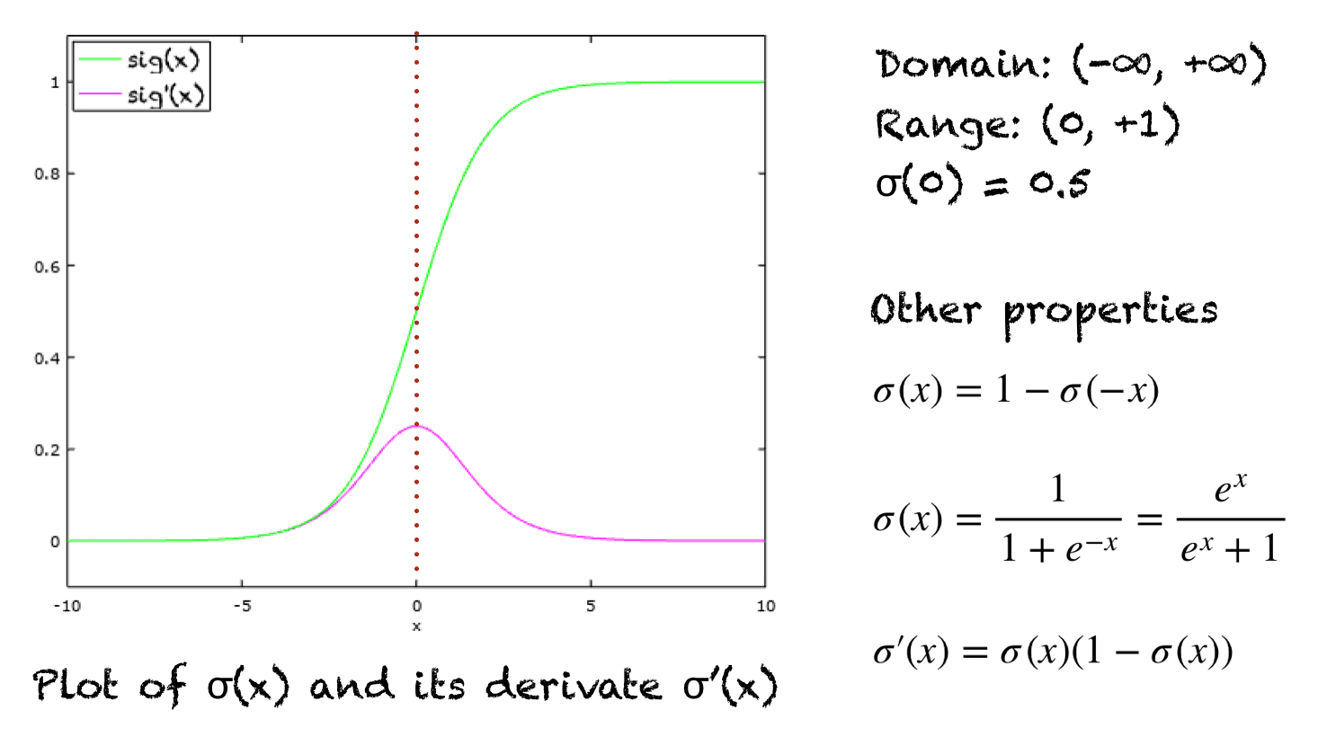
L1[i][j] = dot_prod_res + b1[j]We dont quite have the desired output of this layer’s neurons yet as they also require some form of non-linearity since all we’ve performed so far is a bunch of linear operations in our inputs. This is critical in Neural Networks because without any non-linearity then we’d end up with just a linear transformation of whatever input we put in which is essentially like using a basic (but large) linear function for a specific output, not the complex categorial output we’re after. Instead, it’s this non-linearity which allows these networks to approximate virtually anything. This feature is known as an “activation” of the neuron and it takes the output of what we created above and sends it through a non-linear function, i.e. an Activation Function. There are several different types of activation functions. One of the most well known ones is called the Sigmoid function which squashes the output between 0 and 1 so you can think of a near-zero activation being a neuron that doesn’t “fire” and up near one the neuron is firing. Another activation function, and the one we’ll be using, is called the Rectified Linear Unit or ReLu function which is literally just “If output is above zero, do nothing. Else, make it zero.” Due to this function’s simple calculation and some other important aspects such as faster initial training and avoiding the vanishing gradient problem in networks with more layers (take a look here if you’re curious, but I personally found I obtained an intuative understanding by just analyzing the graph of sigmoid’s derivative which you can see has a large portion of its derivative near zero so of course after several layer-chains of this, the gradient would have a pretty high chance to trend towards zero) in addition to it being used in mordern Machine Learning, we’re going to use it here. The general ReLu definition is given by: \[ \begin{align} ReLu(z) = max(0, z) \end{align} \] So, as you’ve probably already guessed, its forward iterative implementation is super straightforward - just go through all the values in L1 and if a value is below zero, then set it to zero. For readability, we’ll store this result in a new matrix, A1:
#Relu activation - A1
A1 = [[None for i in range(layer1_out)] for j in range(total_train)] #6000 by 32
for i in range(total_train):
    for j in range(layer1_out):
        A1[i][j] = 0 if L1[i][j] <= 0 else L1[i][j]
Our first and only hidden layer is now complete! It’s time for the output layer which is actually extremely similar to the last layer. The output of this layer is defined by: \[ \begin{align} L2 = A1 @ W2 + b2 \end{align} \] This is just another dot product with a bias term. We’ve got our A1 matrix which is the same size as L1, 6000 by 32, and then our W2 matrix which is 32 by 10. So our third nested loop with all the \(A1_i\) times \(W2_i\) will be the 32 and our output matrix will be 6000 by 10, or 6000 sets of 10-size arrays where each 0-9 index relates to the probability the network believes an input image is each 0-9 digit. We code this as follows:
#L2 = A1 @ W2 + b2 (This is our Logits here)
L2 = [[None for i in range(layer2_out)] for j in range(total_train)] #6000 by 10
for i in range(total_train):
    for j in range(layer2_out):
        dot_prod_res = 0
        for k in range(layer2_in):
            dot_prod_res += A1[i][k] * W2[k][j]
        L2[i][j] = dot_prod_res + b2[j]
Now, this output’s range of values can, in theory, be infinite. However they’ll probably be small from how we scaled our data. Let’s take a look at the output of the first image, L2[0]:
print('Network raw output of first image:')
print([round(i, 4) for i in L2[0]])
Network raw output of first image:
[-0.0451, 0.0412, -0.0423, -0.0009, 0.0082, 0.0218, -0.0284, 0.0152, -0.0018, 0.0079]These 10 values do relate to the probability for each 0-9 digit where the highest value is currently which digit this untrained network believes that first image is. So with 0.0412 being the highest, which is index 1, the network thinks the first image is a 1 (and if you noted the labels on our first 10 digits above, it actually is a 1. We totally got lucky lol). Now, this can be difficult to interpret and it’s hard to tell just how confident the network actually thinks it’s a 1. So to make it much easier to interpret (as well as several other aspects we’ll discuss later in this series) there exists something called the Softmax Function: \[ \begin{align} \sigma(z_i) = \frac{e^{z_{i}}}{\sum_{j=1}^n e^{z_{j}}} \end{align} \] Let’s apply it to our first output example, L2[0] above:
softmax_ex = [None]*10 #10 digits, i.e. len(L2[0]) = 10
e_sum = 0
for value in L2[0]:
    e_sum += math.exp(value)
for i in range(10):
    softmax_ex[i] = math.exp(L2[0][i])/e_sum
print('Softmax output of first image:')
print([round(i, 4) for i in softmax_ex])
print(f'The sum of this output is: {sum(softmax_ex)}')
Softmax output of first image:
[0.0958, 0.1044, 0.0961, 0.1001, 0.101, 0.1024, 0.0974, 0.1017, 0.1, 0.101]
The sum of this output is: 1.0As you may have noticed, the Softmax function just converted our outputs into actual probabilities in decimal format which all sum to 1. This is much easier to interpret and we can see that the network isn’t very confident the input image is a 1 since almost all digits are near 10%. This makes sense as we haven’t done any training yet; we simply got lucky from our random initalization.
The Softmax function is most often used on the output layer for classification problems such as this one. Then, a loss function, which is a function that calculates how far off (or close) the network’s output is to the true label, is performed upon this such as the Negative Log Likelihood which compares the true label to the softmax’s output of this same index. Then, being a loss function, we wish to minimize the loss throughout training.
Annnnnd here’s where we’re going to deviate from what should be used for a classification problem such as this. The Softmax function followed by a probability-based loss function comparing it to true labels is the standard approach. Unfortunately, the derivatives of these are fairly complex due to the summation of exponentials and get a little out of hand with our iterative approach. Therefore, we’re going to skip using the awesome Softmax function, meaning that the max value per 10-size array in L2 will be our network prediction. We still need a loss function though! So we’re going to use a very basic one which is typically used for regression problems and is far easier to differentiate: Mean Squared Error (MSE) Loss. The formula for MSE is: \[
\begin{align}
\sum_{i=1}^{n} \frac {1}{n} (x_i-y_i)^2
\end{align}
\] This loss function will increasingly punish values the further away they are from the true answer (because of the square). And since we’ve got a fairly simple classification problem and we’ve scaled inputs to between 0 and 1 with labels that are also 0’s and 1’s, it’ll work okay for our needs. That said, this is not best practice and we’ll use the Softmax with a different loss function in the next part of this series. It just seemed wise to introduce the correct way to solve this problem before going forward with an ill-advised solution. We’ll take another look at the Softmax output since its easy to interpret after we train our network.
So without further ado, we’ll now calculate our loss using MSE:
#Loss - Mean Squared Error to get Predictions
loss = 0
n_mse = total_train*layer2_out
for i in range(total_train):
    for j in range(layer2_out):
        loss += ((L2[i][j] - Y_train[i][j])**2)/n_mse
And with that, we’ve finished our forward pass of the network - we sent in inputs and recevied an output then compared the two to see how accurate we were.
Next up is the difficult part, which is the backward pass for the network to improve. The backward pass through the network is what will give us the gradients of our weights and biases; or in an easier to understand lingo, we’re going to figure out just how much changing our weights and biases will effect the final output. This is essentially an instantaneous rate of change for W1/W2/b1/b2 effecting our Loss. A mathematical name to describe an instantaneous rate of change of a function is called its derivative. So yes, hopefully “derivative” isn’t a scary word because we’re going to find the derivatives of our weights and biases with respect to the Loss. This is all in an effort to minimize our Loss because the lower our Loss, then the closer each of the network’s predictions are to the target. So if we find each of these derivatives and then subtract a portion of them from their respective weight/bias then we will create a more accurate network for our classification problem; i.e. our network will “learn”. This is called Gradient Descent and then going backward through the network calculating the derivatives of everything with respect to the Loss is called Backpropagation.
To calculate these derivatives for Backpropagation, we must use the Chain Rule. An example of the Chain Rule is as follows: \[ \begin{align} \frac{dz}{{dx}} = \frac{dz}{{dy}}\cdot\frac{{dy}}{{dx}} \end{align} \]
We can apply this rule to find our derivates of W1, W2, b1, and b2 with respect to the Loss. Which means we will be going backwards through our “L1 –> A1 –> L2 –> Loss” chain. If we go through the chain in reverse, we will find that our derivates of the weights and biases with respect to the Loss can be calulated from the following chain of local derivatives: \[ \begin{align} & \frac{dLoss}{{dW2}} = \frac{dLoss}{{dL2}}\cdot\frac{{dL2}}{{dW2}}\\ & \frac{dLoss}{{db2}} = \frac{dLoss}{{dL2}}\cdot\frac{{dL2}}{{db2}}\\ & \frac{dLoss}{{dW1}} = \frac{dLoss}{{dL2}}\cdot\frac{{dL2}}{{dA1}}\cdot\frac{{dA1}}{{dL1}}\cdot\frac{{dL1}}{{dW1}}\\ & \frac{dLoss}{{db1}} = \frac{dLoss}{{dL2}}\cdot\frac{{dL2}}{{dA1}}\cdot\frac{{dA1}}{{dL1}}\cdot\frac{{dL1}}{{db1}} \end{align} \] The left-to-right order of these chains above is the backward order through our network. So let’s start with \(\frac{dLoss}{{dL2}}\). In our forward pass, for L2, we had: \[ \begin{align} Loss = \sum_{i=1}^{n\_mse}\frac{1}{n\_mse}(L2_{i}-Ytrain_{i})^2 \end{align} \] And then its derivative with respect to L2 is: \[ \begin{align} \frac{dLoss}{{dL2}} = \sum_{i=1}^{n\_mse}\frac{2}{n\_mse}(L2_{i}-Ytrain_{i}) \end{align} \] In the forward pass, we calculated the total MSE over all training examples to obtain a single Loss value. Here we want the derivative for each training example so we need to obtain a 6000 by 10 matrix meaning we are not going to perform the summation:
#dLoss_dL2 is mse derivative
dLoss_dL2 = [[None for i in range(layer2_out)] for j in range(total_train)] #6000 by 10
for i in range(total_train):
    for j in range(layer2_out):
        dLoss_dL2[i][j] = ((2)/(n_mse))*(L2[i][j]-Y_train[i][j])
To obtain \(\frac{dLoss}{{dW2}}\) we’ll need \(\frac{dL2}{{dW2}}\) and to multiply them together. For \(\frac{dL2}{{dW2}}\) we are finding the derivative of \(W2\) with respect to \(L2\) in the equation: \[ \begin{align} L2 = A1 @ W2 + b2 \end{align} \] If you go through the steps of the above dot product and eliminate variables W2 and b2 as you would in deriving you would find the following: \[ \begin{align} \frac{dL2}{{dW2}} = {A1}^T \end{align} \] Yes, to find our \(\frac{dL2}{{dW2}}\) we are performing a transpose of \(A1\). \(A1\) was a 6000 by 32 matrix and so we’re writing it to a new 32 by 6000 matrix:
#dL2_dW2 is A1 transpose
dL2_dW2 = [[None for i in range(total_train)] for j in range(layer2_in)] #32 by 6000
for i in range(layer2_in):
    for j in range(total_train):
        dL2_dW2[i][j] = A1[j][i]
Now, thinking intuatively, to calculate \(\frac{dLoss}{{dW2}}\) we have a 6000 by 10 matrix and a 32 by 6000 matrix and need a 32 by 10 matrix (the size of \(W2\)). We can get this by performing the dot product of \(\frac{dL2}{{dW2}}@\frac{dLoss}{{dL2}}\) which will eliminate the inner 6000 dimension and leave us with a 32 by 10 matrix:
#dLoss_dW2 = dLoss_dL2*dL2_dW2
dLoss_dW2 = [[None for i in range(layer2_out)] for j in range(layer2_in)] #32 by 10
for i in range(layer2_in):
    for j in range(layer2_out):
        dot_prod_res = 0
        for k in range(total_train):
            dot_prod_res += dL2_dW2[i][k]*dLoss_dL2[k][j]
        dLoss_dW2[i][j] = dot_prod_res
To find \(\frac{dLoss}{{db2}}\) we need \(\frac{dL2}{{db2}}\) which appears equal to 1 looking at the equation for \(L2\). However, if we look through our iterative calculation of \(L2\) we are adding each \(b2_j\) along dimension 10 for every 6000 training example meaning that (because addition’s derivative is just 1) \(\frac{dL2}{{db2}}\) is actually a 1 by 6000 matrix full of 1’s. So to end up with \(\frac{dLoss}{{db2}}\) being a 1 by 10 (the size of \(b2\)) we must perform the dot product \(\frac{dL2}{{db2}}@\frac{dLoss}{{dL2}}\) (1 by 6000 @ 6000 by 10) which is actually the same as summing all the columns of \(\frac{dLoss}{{dL2}}\) to get our 1 by 10:
#dLoss_db2 = dLoss_dL2*dL2_db2
#dL2_db2 = [[1]]*6000
#dLoss_db2 = dLoss_dL2, but b2 is broadcasted, so to get back to
#            a 1 by 10 size matrix, we must sum the columns.
dLoss_db2 = [0 for i in range(layer2_out)] #1 by 10
for i in range(layer2_out):
    for j in range(total_train):
        dLoss_db2[i] += dLoss_dL2[j][i]
Nice work, we found \(\frac{dLoss}{{dW2}}\) and \(\frac{dLoss}{{db2}}\) and its time to find \(\frac{dLoss}{{dW1}}\) and \(\frac{dLoss}{{db1}}\) which have a larger chain. Continuing with left-to-right in our chain, we need to find \(\frac{dL2}{{dA1}}\). Lucky for us, this is the same calculation as when we found \(\frac{dL2}{{dW2}}\) only now instead of grabbing the transpose of \(A1\) we’re finding the transpose of \(W2\) which is a 10 by 32 matrix:
#dL2_dA1 is W2 transpose
dL2_dA1 = [[None for i in range(layer2_in)] for j in range(layer2_out)] #10 by 32
for i in range(layer2_out):
    for j in range(layer2_in):
        dL2_dA1[i][j] = W2[j][i]
Easy. Next up in our chain is \(\frac{dA1}{{dL1}}\) which is the derivative of our ReLu activation function. This derivative is also quite simple and is essentially “If value in \(A1\) is 0, then the derivative is 0, else the derivative is 1”. This also shows why ReLu is a popular activation function as its derivative is simple with low computation. Our \(\frac{dA1}{{dL1}}\) is then a 6000 by 32 matrix:
#dA1_dL1 -- > Relu derivative
dA1_dL1 = [[None for i in range(layer1_out)] for j in range(total_train)] #6000 by 32
for i in range(total_train):
    for j in range(layer1_out):
        dA1_dL1[i][j] = 0 if A1[i][j] <= 0 else 1
Next we need to find our last two local derivatives \(\frac{dL1}{{dW1}}\) and \(\frac{dL1}{{db1}}\). Similar to \(\frac{dL2}{{dW2}}\), \(\frac{dL1}{{dW1}}\) is the transpose of \(Xtrain\) which gives us a 784 by 6000 matrix:
#dL1_dW1 is x transpose 4x5
dL1_dW1 = [[None for i in range(total_train)] for j in range(layer1_in)] #784 by 6000
for i in range(layer1_in):
    for j in range(total_train):
        dL1_dW1[i][j] = X_train[j][i]
And for \(\frac{dL1}{db1}\) we can see from the equation for \(L1\) that this derivative is 1. However, once again we must find the shape of this. In the forward pass we’re adding \(b1\) along dimension 32 for all 6000 training examples. And since this add-along-32 has a derivative of 1, just like with \(\frac{dL1}{db2}\) our derivative is also a 1 by 6000 matrix of 1’s. We’ll just note this for now.
With all our local derivative complete, we can multiply together the chains. We just have to keep in mind the dimensions of each so we perform the correct multiplication of terms. Starting with \(\frac{dLoss}{dL2}\cdot\frac{dL2}{dA1}\) we see we have a 6000 by 10 matrix times a 10 by 32 matrix. Thus, we have a dot product with a 6000 by 32 resultant matrix: \[ \begin{align} \frac{dLoss}{dA1} = \frac{dLoss}{dL2}@\frac{dL2}{dA1} \end{align} \] Coding this up is straight forward now that we’re practiced:
#dLoss_dA1 = dLoss_dL2*dL2_dA1
dLoss_dA1 = [[None for i in range(layer2_in)] for j in range(total_train)] #6000 by 32
for i in range(total_train):
    for j in range(layer2_in):
        dot_prod_res = 0
        for k in range(layer2_out):
            dot_prod_res += dLoss_dL2[i][k]*dL2_dA1[k][j]
        dLoss_dA1[i][j] = dot_prod_res
Next is to multiply in \(\frac{dA1}{dL1}\) which is also a 6000 by 32 size matrix so we have a straight forward element-wise multiplcation to get \(\frac{dLoss}{dL1}\):
#dLoss_dL1 = dLoss_dA1*dA1_dL1
dLoss_dL1 = [[None for i in range(layer1_out)] for j in range(total_train)] #6000 by 32
for i in range(total_train):
    for j in range(layer1_out):
        dLoss_dL1[i][j] = dLoss_dA1[i][j]*dA1_dL1[i][j]
And finally, to get our \(\frac{dLoss}{dW1}\) we must multiply \(\frac{dLoss}{dL1}\) by \(\frac{dL1}{dW1}\) which is a 784 by 6000 matrix. To end up with our final 784 by 32 sized matrix we need to perform another dot product: \[ \begin{align} \frac{dLoss}{dW1} = \frac{dL1}{dW1}@\frac{dLoss}{dL1} \end{align} \] Which is a 784 by 6000 times a 6000 by 32, meaning the middle dimension will be eliminated:
#dLoss_dW1 = dLoss_dL1*dL1_dW1
dLoss_dW1 = [[None for i in range(layer1_out)] for j in range(layer1_in)] #784 by 32
for i in range(layer1_in):
    for j in range(layer1_out):
        dot_prod_res = 0
        for k in range(total_train):
            dot_prod_res += dL1_dW1[i][k]*dLoss_dL1[k][j]
        dLoss_dW1[i][j] = dot_prod_res
Last, but not least, is \(\frac{dLoss}{db1}\) which we get with \(\frac{dLoss}{dL1}\) times \(\frac{dL1}{db1}\). We noted previously that \(\frac{dL1}{db1}\) is a 1 by 6000 matrix of 1’s. So to get our 1 by 32 matrix, \(\frac{dLoss}{db1}\), we have a final dot product: \[ \begin{align} \frac{dLoss}{db1} = \frac{dL1}{db1}@\frac{dLoss}{dL1} \end{align} \] Which is a 1 by 6000 times a 6000 by 32. And just like with b2, calculating this is the same as summing the columns of \(\frac{dLoss}{dL1}\):
#dLoss_b1 = dLoss_dL1*dL1_db1
#dL1_db1 = [[1]]*6000
#dLoss_db1 = dLoss_dL1, but b1 is broadcasted, so to get back to a [7]
#        size matrix, we must sum the columns
dLoss_db1 = [0 for i in range(layer1_out)]
for i in range(layer1_out):
    for j in range(total_train):
        dLoss_db1[i] += dLoss_dL1[j][i]
And there we have it! Backpropagation through our simple network. It turned out to be quite a bit of tedious work, however by performing this tedious task, we’ve learned another in-depth part of how Neural Networks actually work. Plus, we gain even more appreciation for some of the things to come in this series such as vectorized solutions and autograd libraries.
Now that we’ve found our gradients, its time to make it so our network can actually learn. If you watched 3Blue1Brown’s video on Gradient Descent then this is what we’re now implementing. We are going to subtract a portion of each term in the gradient from their respective term in the weights and biases. We do this using what’s called a Learning Rate, typically denoted \(lr\), which is different depending on the network. Usually, this rate value is small and is often desired to get smaller as the network learns. In our case, with our relatively small, simple, and iterative network the goal is to hit a decent accuracy of the Test Set as quick as possible because with this iterative approach learning is going to take a long time. So through some trial-and-error using Pytorch it takes about 300 full iterations forward and backward through the network with a learning rate of 0.8 to achieve ~90% accuracy on the Test Set. With this, to make our network learn we subtract 0.8 times each gradient term from its equivalent weight or bias term:
#Learn:
lr = 0.8
for i in range(layer1_in):
    for j in range(layer1_out):
        W1[i][j] += -lr*dLoss_dW1[i][j]
for i in range(layer1_out):
    b1[i] += -lr*dLoss_db1[i]
for i in range(layer2_in):
    for j in range(layer2_out):
        W2[i][j] += -lr*dLoss_dW2[i][j]
for i in range(layer2_out):
    b2[i] += -lr*dLoss_db2[i]
Now we can combine everything to create what’s called our training loop. It is very possible to make all our iterative code much more efficient by reducing iterations through combining some of the for loops. However, for educational purposes we’re going to leave it all as-is so its easily followed. We’re going to run 300 iterations which should get us to about 90% accuracy, however it’s going to take along time so let’s use Python’s timer library to see how long it takes overnight. Actually, since we’re training on all the data being used during every iteration (we will explore “batching” data later in this series), that is called an Epoch. An Epoch is just a counter for when all the training data has been fed into the network which is useful when batching smaller chunks of training data at a time. So let’s perform 300 Epochs and see how long it takes:
start = timer()

for _ in range(300):
    #---forward---
    #L1 = X_train @ W1 + b1
    L1 = [[None for i in range(layer1_out)] for j in range(total_train)]
    for i in range(total_train):
        for j in range(layer1_out):
            dot_prod_res = 0
            for k in range(layer1_in):
                dot_prod_res += X_train[i][k] * W1[k][j]
            L1[i][j] = dot_prod_res + b1[j]
    #Relu activation - A1
    A1 = [[None for i in range(layer1_out)] for j in range(total_train)]
    for i in range(total_train):
        for j in range(layer1_out):
            A1[i][j] = 0 if L1[i][j] <= 0 else L1[i][j]
    #L2 = A1 @ W2 + b2 (This is our Logits here)
    L2 = [[None for i in range(layer2_out)] for j in range(total_train)]
    for i in range(total_train):
        for j in range(layer2_out):
            dot_prod_res = 0
            for k in range(layer2_in):
                dot_prod_res += A1[i][k] * W2[k][j]
            L2[i][j] = dot_prod_res + b2[j]
    #Loss - Mean Squared Error to get Predictions
    loss = 0
    total_vals_out = total_train*layer2_out
    for i in range(total_train):
        for j in range(layer2_out):
            loss += ((L2[i][j] - Y_train[i][j])**2)/total_vals_out

    #---backward---
    #dLoss_dL2 is mse derivative
    dLoss_dL2 = [[None for i in range(layer2_out)] for j in range(total_train)]
    for i in range(total_train):
        for j in range(layer2_out):
            dLoss_dL2[i][j] = ((2)/(n_mse))*(L2[i][j]-Y_train[i][j])
    #dL2_dW2 is A1 transpose
    dL2_dW2 = [[None for i in range(total_train)] for j in range(layer2_in)]
    for i in range(layer2_in):
        for j in range(total_train):
            dL2_dW2[i][j] = A1[j][i]
    #dLoss_dW2 = dLoss_dL2*dL2_dW2
    dLoss_dW2 = [[None for i in range(layer2_out)] for j in range(layer2_in)]
    for i in range(layer2_in):
        for j in range(layer2_out):
            dot_prod_res = 0
            for k in range(total_train):
                dot_prod_res += dL2_dW2[i][k]*dLoss_dL2[k][j]
            dLoss_dW2[i][j] = dot_prod_res
    #dLoss_db2 = dLoss_dL2*dL2_db2
    dLoss_db2 = [0 for i in range(layer2_out)]
    for i in range(layer2_out):
        for j in range(total_train):
            dLoss_db2[i] += dLoss_dL2[j][i]
    #dL2_dA1 is W2 transpose
    dL2_dA1 = [[None for i in range(layer2_in)] for j in range(layer2_out)]
    for i in range(layer2_out):
        for j in range(layer2_in):
            dL2_dA1[i][j] = W2[j][i]
    #dA1_dL1 -- > Relu derivative
    dA1_dL1 = [[None for i in range(layer1_out)] for j in range(total_train)]
    for i in range(total_train):
        for j in range(layer1_out):
            dA1_dL1[i][j] = 0 if A1[i][j] <= 0 else 1
    #dL1_dW1 is x transpose 4x5
    dL1_dW1 = [[None for i in range(total_train)] for j in range(layer1_in)]
    for i in range(layer1_in):
        for j in range(total_train):
            dL1_dW1[i][j] = X_train[j][i]
    #dLoss_dA1 = dLoss_dL2*dL2_dA1
    dLoss_dA1 = [[None for i in range(layer2_in)] for j in range(total_train)]
    for i in range(total_train):
        for j in range(layer2_in):
            dot_prod_res = 0
            for k in range(layer2_out):
                dot_prod_res += dLoss_dL2[i][k]*dL2_dA1[k][j]
            dLoss_dA1[i][j] = dot_prod_res
    #dLoss_dL1 = dLoss_dA1*dA1_dL1
    dLoss_dL1 = [[None for i in range(layer1_out)] for j in range(total_train)]
    for i in range(total_train):
        for j in range(layer1_out):
            dLoss_dL1[i][j] = dLoss_dA1[i][j]*dA1_dL1[i][j]
    #dLoss_dW1 = dLoss_dL1*dL1_dW1
    dLoss_dW1 = [[None for i in range(layer1_out)] for j in range(layer1_in)]
    for i in range(layer1_in):
        for j in range(layer1_out):
            dot_prod_res = 0
            for k in range(total_train):
                dot_prod_res += dL1_dW1[i][k]*dLoss_dL1[k][j]
            dLoss_dW1[i][j] = dot_prod_res
    #dLoss_b1 = dLoss_dL1*dL1_db1
    dLoss_db1 = [0 for i in range(layer1_out)]
    for i in range(layer1_out):
        for j in range(total_train):
            dLoss_db1[i] += dLoss_dL1[j][i]

    #Learn:
    lr = 0.8
    for i in range(layer1_in):
        for j in range(layer1_out):
            W1[i][j] += -lr*dLoss_dW1[i][j]
    for i in range(layer1_out):
        b1[i] += -lr*dLoss_db1[i]
    for i in range(layer2_in):
        for j in range(layer2_out):
            W2[i][j] += -lr*dLoss_dW2[i][j]
    for i in range(layer2_out):
        b2[i] += -lr*dLoss_db2[i]

    #Print every 10 Epochs
    if _%10 == 0 or _ == 299:
        print(f'Epoch: {_}\n\tLoss: {loss}')
end = timer()
print(f'Total time for 300 Epochs: {end - start} seconds.')
Epoch: 0
Loss: 0.08847381438371525
Epoch: 10
Loss: 0.07941663402576407
Epoch: 20
Loss: 0.05853325970911123
Epoch: 30
Loss: 0.05148405639645048
Epoch: 40
Loss: 0.04664412083181115
Epoch: 50
Loss: 0.04273779754470685
Epoch: 60
Loss: 0.0405243776626876
Epoch: 70
Loss: 0.03875570757224373
Epoch: 80
Loss: 0.036854907083257775
Epoch: 90
Loss: 0.035321623248538325
Epoch: 100
Loss: 0.03404829810194227
Epoch: 110
Loss: 0.03293688470078946
Epoch: 120
Loss: 0.031948822194692056
Epoch: 130
Loss: 0.031060419461079878
Epoch: 140
Loss: 0.030254934045411623
Epoch: 150
Loss: 0.029523032980928652
Epoch: 160
Loss: 0.028851990081670276
Epoch: 170
Loss: 0.028230829995408734
Epoch: 180
Loss: 0.02765606265763907
Epoch: 190
Loss: 0.02711831362105811
Epoch: 200
Loss: 0.026615757159766558
Epoch: 210
Loss: 0.02614325249029197
Epoch: 220
Loss: 0.025697375844800578
Epoch: 230
Loss: 0.025277634231562554
Epoch: 240
Loss: 0.02488321578396466
Epoch: 250
Loss: 0.02451023120767074
Epoch: 260
Loss: 0.024161968709304215
Epoch: 270
Loss: 0.023843686092740075
Epoch: 280
Loss: 0.023532022940507418
Epoch: 290
Loss: 0.023226961127444684
Epoch: 299
Loss: 0.022960782444860155
Total time for 300 Epochs: 21836.3504608 seconds.About 6 hours! That’s a very long time compared to the vectorized solutions we’ll do in the future. However, this is working exactly as expected and our loss is going down after each Epoch. If we trained for longer we could get this even lower, we just dont want to overfit to our training data which will make our network poorly respond to unseen data. That said, let’s see how well our, now trained, network compares against the Test Set. To find this, first we simply perform the same Forward pass, but this time we use \(Xtest\) rather than \(XTrain\):
#Check against the test set:
total_test = len(X_test)
L1_test = [[None for i in range(layer1_out)] for j in range(total_test)]
A1_test = [[None for i in range(layer1_out)] for j in range(total_test)]
#L1 & A1 combined:
for i in range(total_test):
    for j in range(layer1_out):
        dot_prod_res = 0
        for k in range(layer1_in):
            dot_prod_res += X_test[i][k] * W1[k][j]
        L1_test[i][j] = dot_prod_res + b1[j]
        A1_test[i][j] = 0 if L1_test[i][j] <= 0 else L1_test[i][j]
#L2 = A1 @ W2 + b2
L2_test = [[None for i in range(layer2_out)] for j in range(total_test)]
for i in range(total_test):
    for j in range(layer2_out):
        dot_prod_res = 0
        for k in range(layer2_in):
            dot_prod_res += A1_test[i][k] * W2[k][j]
        L2_test[i][j] = dot_prod_res + b2[j]
Now we can take the \(L2test\) results above and compare the maximum index of each to its respective \(Ytest\) max index:
#Compare the index with maximum value per test example:
correct = 0
incorrect_idxs = [] #Store these for later
for test_num in range(total_test):
    Y_test_maxindex = Y_test[test_num].index(max(Y_test[test_num]))
    L2_maxindex = L2_test[test_num].index(max(L2_test[test_num]))
    if Y_test_maxindex == L2_maxindex:
        correct += 1
    else:
        incorrect_idxs.append((test_num, L2_maxindex))
print(f'\tTest Set Accuracy = {(correct/total_test)*100}%')
Test Set Accuracy = 89.9%Accuracy of ~90%! Not bad for no external libraries and from complete scratch!
Let’s briefly look at the SoftMax output again on our first training example as well as our first test example:
#SoftMax of X_train[0]:
softmax_ex2 = [None]*10
e_sum = 0
for value in L2[0]:
    e_sum += math.exp(value)
for i in range(10):
    softmax_ex2[i] = math.exp(L2[0][i])/e_sum
#SoftMax of X_test[0]:
softmax_ex2_test = [None]*10
e_sum = 0
for value in L2_test[0]:
    e_sum += math.exp(value)
for i in range(10):
    softmax_ex2_test[i] = math.exp(L2_test[0][i])/e_sum
#Add img plots along with output:
%matplotlib inline
img_data = []
last = 0
fig = plt.figure(figsize=(1, 1))
for j in range(int(img_pxs**0.5), img_pxs + 1, int(img_pxs**0.5)):
    img_data.append(X_train[0][last:j])
    last = j
plt.imshow(img_data, cmap="gray")
plt.title(f'1st Train Label: {Y_train[0].index(max(Y_train[0]))}')
plt.axis('off')
plt.show();
print('Softmax output of first training example:')
print([round(i, 4) for i in softmax_ex2])
img_data = []
last = 0
fig = plt.figure(figsize=(1, 1))
for j in range(int(img_pxs**0.5), img_pxs + 1, int(img_pxs**0.5)):
    img_data.append(X_test[0][last:j])
    last = j
plt.imshow(img_data, cmap="gray")
plt.title(f'1st Test Label: {Y_test[0].index(max(Y_test[0]))}')
plt.axis('off')
plt.show();
print('Softmax output of first test example:')
print([round(i, 4) for i in softmax_ex2_test])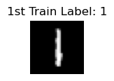
Softmax output of first training example:
[0.088, 0.2312, 0.0909, 0.0815, 0.0865, 0.0894, 0.0853, 0.0844, 0.0813, 0.0815]
Softmax output of first test example:
[0.0901, 0.0964, 0.0914, 0.0862, 0.0907, 0.0789, 0.0957, 0.1112, 0.0989, 0.1606]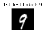
As we can see for our first training example, the index location 1 (which is also our correct label) has a much higher probability output now sitting at 23% confidence meaning our network most definitely improved through training. And then for the unseen test data, index 9 is high which is correct, however index 7 is the second highest which makes sense when you compare the shapes of 9’s and 7’s.
Actually, let’s now take a look at the first 20 incorrect predictions of our trained network:
%matplotlib inline
import matplotlib.pyplot as plt
fig, axes = plt.subplots(nrows= 2, ncols=10, figsize=(8, 8))
fig.tight_layout(h_pad=-41, w_pad=-2)
row_num = 0
col_num = 0
for incorrect in incorrect_idxs[0:20]: #Stored from earlier
    if col_num == 10:
        row_num = 1
        col_num = 0
    idx, pred_label = incorrect
    data_test = []
    last = 0
    for j in range(int(img_pxs**0.5), img_pxs + 1, int(img_pxs**0.5)):
        data_test.append(X_test[idx][last:j])
        last = j
    axes[row_num][col_num].imshow(data_test, cmap="gray")
    axes[row_num][col_num].axis('off')
    axes[row_num][col_num].set_title(pred_label)
    col_num += 1
print('First 20 incorrect labels and images:')
plt.show()
First 20 incorrect labels and images: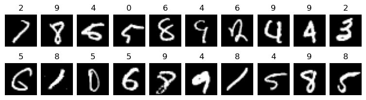
Those aren’t the easiest digits to read, even for humans. But we can see how 4’s and 9’s can be difficult and any oddly shaped digit can be misinterpretted by our very small and simple network. Later, we’ll perform new techniques which will greatly increase our network’s capabilities… even beyond humans.
Finally, as a small aside, if we want to save our network for later we can store all the data into a Dictionary and then use Python’s pickle library to write it to a pickle file:
import pickle
MNIST_Network = {'W1': W1,
                 'b1': b1,
                 'W2': W2,
                 'b2': b2}
with open('MNIST_Network.pickle', 'wb') as handle:
    pickle.dump(MNIST_Network, handle, protocol=pickle.HIGHEST_PROTOCOL)
Then, at a later time after we close down and remove the weight/bias variables from memory, we can read this file to use or even further train our network:
with open('MNIST_Network.pickle', 'rb') as handle:
    Loaded_network = pickle.load(handle)
print(f'W1[0][0:4]: \t{Loaded_network["W1"][0][0:4]}')
print(f'b1[0:4]: \t{Loaded_network["b1"][0:4]}')
print(f'W2[0][0:4]: \t{Loaded_network["W2"][0][0:4]}')
print(f'b2[0:4]: \t{Loaded_network["b2"][0:4]}')
W1[0][0:4]: [-0.026728772284180698, 0.034643550081185664, 0.017772138105435417, 0.020509058949632827]
b1[0:4]: [0.040651823249868504, 0.0967657288695644, 0.019974871602575037, 0.06427076106765985]
W2[0][0:4]: [0.0552450524383754, -0.10533068961436158, 0.04651506974334741, 0.08529839152600965]
b2[0:4]: [0.09277626993915575, 0.1105437252196011, 0.09194765254410657, 0.029433292509831406]And that’s it! A fundamental introduction to Neural Networks. Next up we will be solving the same handwritten digits problem, but using the popular linear algebra library Numpy which will vectorize everything for a substantial improvement on training speed. We will also create a larger network, use all the data, and explore the aforementioned Softmax. So check out the next walkthrough!